Displacement Mapping of the 2025 Myanmar Earthquake using Sentinel-1 SAR Images

Introduction

The aim of the study is to generate a displacement map from Sentinel-1 SAR images and this would help reveal the major ground movement caused by the earthquake and extracts distance information plate shift within the region.

Study Area

The study area selected to generate a displacement map was a big earthquake event that happened in Myanmar, Thailand on 28th March, 2025 with a magnitude of 7.7. According to Wikipedia, the earthquake event is recorded as the most powerful earthquake to strike Myanmar since 1912 and the second deadliest in Myanmar modern history.

Fig 1.0 Collapsed building in Mandalay city in Myanmar, Thailand. Source: BBC News

My motivation behind generating the displacement map for this event is based on my curiosity to understand the effect of the event in the area after I got the news on 29th March, 2025 that one of my colleague that we worked together in Nigeria relocated to the Thailand and it was announced by the HR to send some heartfelt message to her because the earthquake happened close to the area she relocated to.

Fig 1.1 Myanmar City, Thailand on OpenStreetMap

Data Preparation

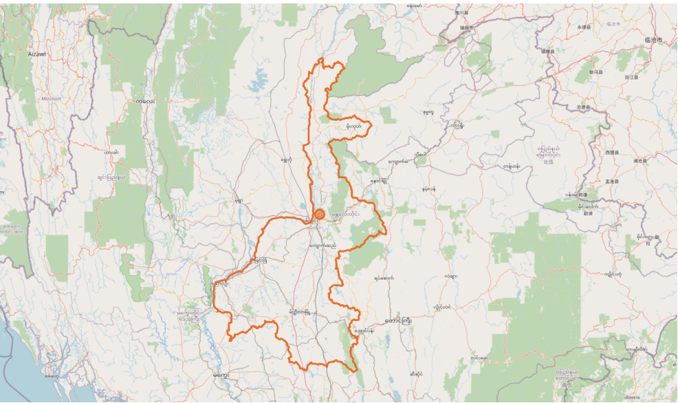
A good number of records of earthquakes can be assessed from the USGS Earthquake Catalog and the map shows the exact location coordinate the event occurred. To obtain the exact location the event happened in Myanmar, I used the search settings by modifying the date and time to start: 2025-03-01 00:00:00 and end: 2025-04-08 23:59:59, selected 4.5+ as the minimum magnitude and applied a custom bounding box within Thailand.

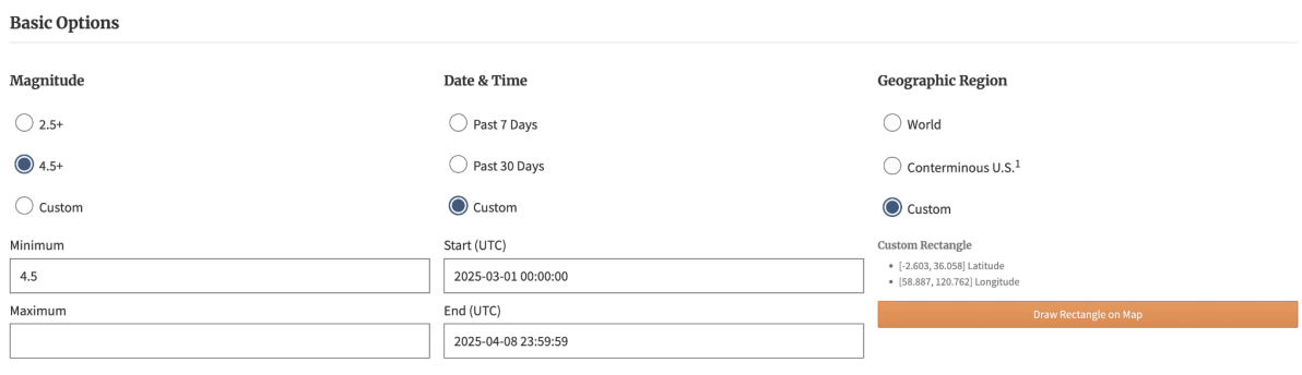
Fig 2.0 USGS Earthquake search settings

After the search was filtered, the first result was the event and it has an epicenter location of 22.011°N 95.936°E.

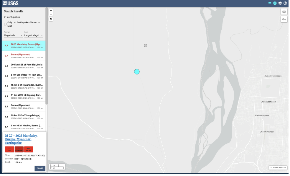
Fig 2.1 Search Result: M 7.7, 2025 Mandalay, Burma (Myanmar) Earthquake

To conduct the Analysis, I used the point coordinate in ASF Data Search website to parameters selected date range starting from 27.03.2025 to 04.13.2025.

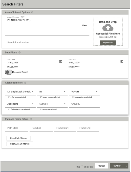
Fig 2.0 ASF Data search filter to download Sentinel-1 InSAR for the Study Area.

Only three Sentinel-1 Products were available within the time range and the study site. I downloaded the scene before the earthquake which was acquired on 27th, March 2025:

S1A_IW_SLC__1SDV_20250327T114746_20250327T114813_058490_073C5E_FF9E

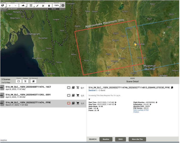
Fig 2.2 Selection of Sentinel-1 C-Band Product before the earthquake event

Afterwards, to ensure the displacement map can clearly be captured after the analysis, I downloaded the products of the same swath days after the earthquake event which was on 8th April, 2025:

S1A_IW_SLC__1SDV_20250408T114746_20250408T114813_058665_07438A_16C7

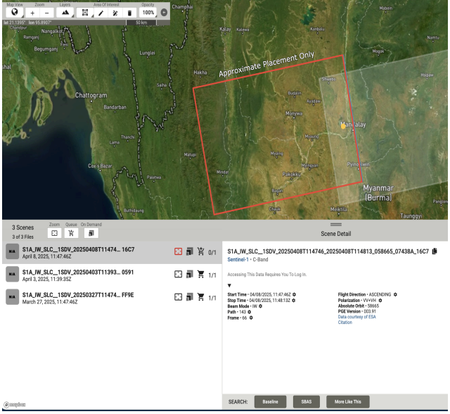
Fig 2.3 Selection of Sentinel-1 C-Band Product after the earthquake event

Image Type	Date of Acquisition	Relation to Event
Primary	27.03.2025	1 day before the Earthquake
Secondary	08.04.2025	11 days after the Earthquake
Temporal Baseline	12 Days	Short Baseline

Table 2.0 Temporal Baseline information based on product selection

Methodology

Interferometric analysis was used to analyze the displacement caused by the earthquake. This technique exploits the phase difference between the two complex SAR images covering the earthquake epicenter, acquired from the same sensor positions at different times (repeat-pass interferometry). By comparing these observations, it can be used to extract precise information regarding changes in the Earth's terrain and surface displacement with millimeter-to-centimeter accuracy.

Software Used

Two applications were used. The first main was the Sentinel Application Platform (SNAP) by the European Space Agency which I used to perform the interferometry analysis and is a common architecture for all Sentinel Toolboxes and Google Earth Pro application was used the visualize the exported displacement map to visualize the displaced region with the google satellite image of earthquake epicentre in Myanmar, Thailand.

Result

These are the steps followed to generate the displacement map using SNAP.

Step 1 — Split the Subswath

I loaded the two Sentinel-1 SLC images that were downloaded into SNAP with unzipping the files, and proceeded to perform Split on image by using S-1 TOPS Split.

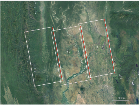
Fig 3.0 Subswath from the Sentinel-1 Images

The following parameter were used to perform the subswath split on the before and after images:

• Subswath — IW1
• Polarization — VV
• Burst — Selected the burst that covered my area of interest

I renamed the output file to reduce the long name and for easy identification of the result.

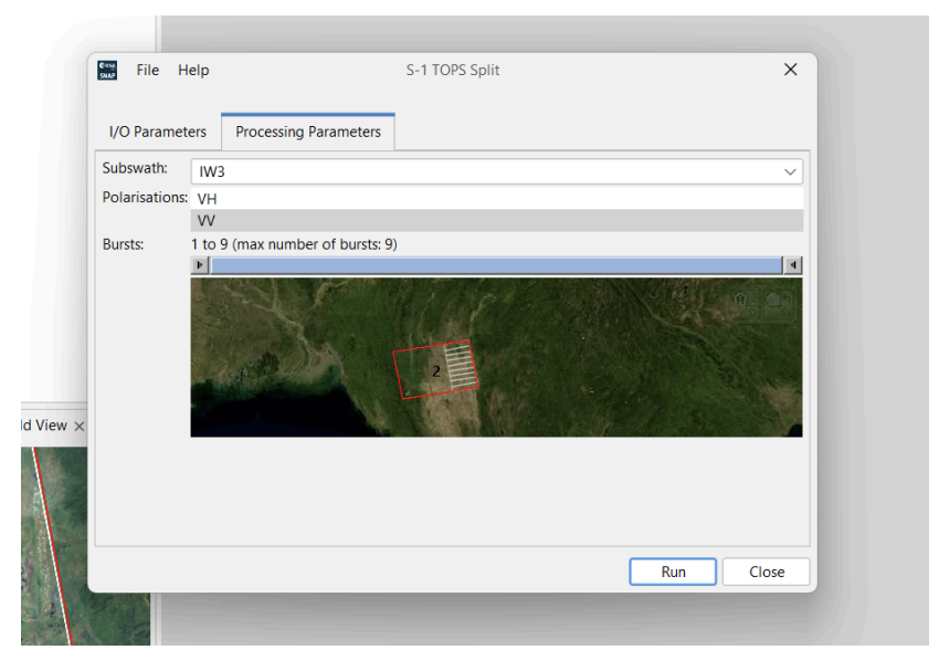
Fig 3.1 Parameters selection to perform Split

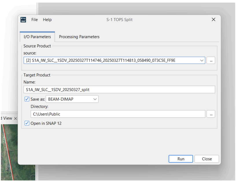
Fig 3.2 Split Process for the Before event Image

Step 2 — Apply Orbit File To Splits

This next process was used to correct the satellite positioning errors of the image. I used the Apply orbit file tool on the split results of both images.

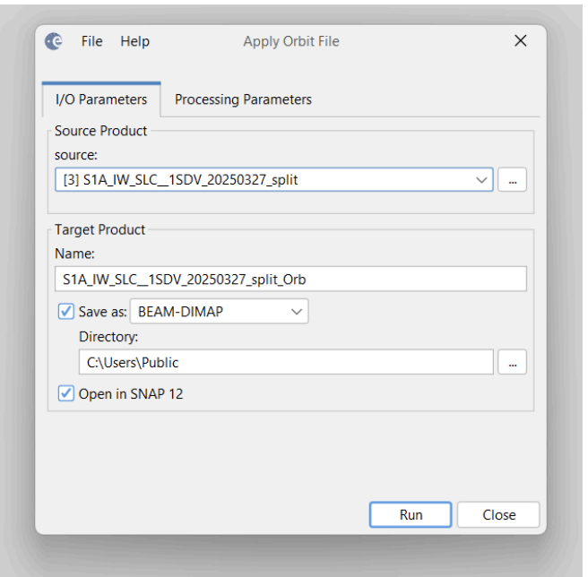
Fig 3.2 Applying Orbit File on Before event Split image

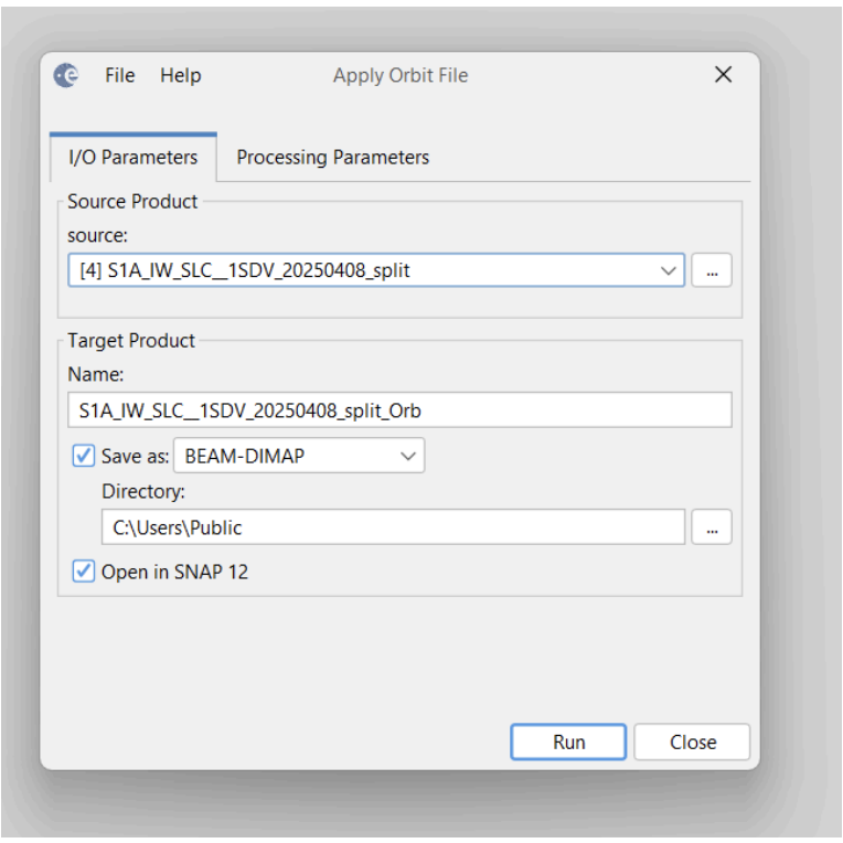
Fig 3.3 Applying Orbit File on After event Split image

Step 3 — Coregistration (Back-Geocoding)

Back-Geocoding was used to co-register the reference and the secondary results after a complete application of the orbit file on the two image splits. This process helps to align the images together. I added the reference and secondary image into the productset reader respectively.

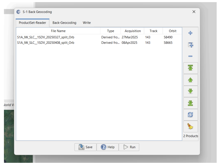
Fig 3.4 Arrangement of Reference and Secondary product using the Product-set Reader interface

I configured the following parameters; At first, I changed the Digital Elevation Model to "SRTM 1Sec HGT (Auto Download)" and checked "Mask out areas with no elevation".

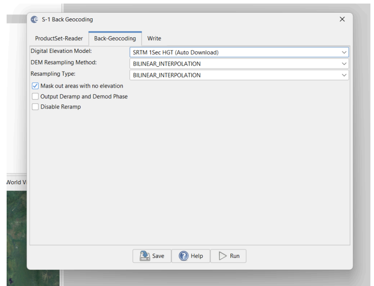
Fig 3.5 Configuring Back-geocoding parameters

Step 4 — Coregistration (Enhanced Spectral Diversity)

This process is optional for the generation of the interferogram. It performs the joint co-registration of a Sentinel-1 stack by creating a network (graph) of images and then estimating range and azimuth offsets by solving an optimization problem. To perform this process, I used the stack file from the back-geocoding result.

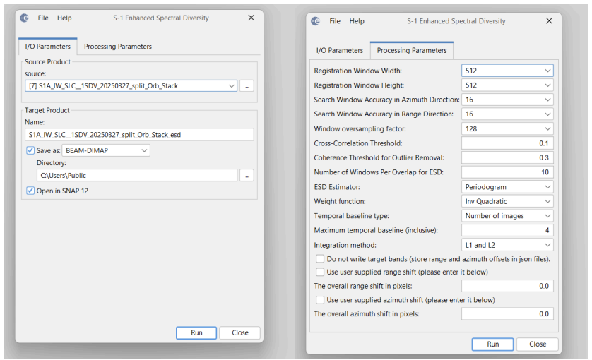
Fig 3.6 Configuring Enhanced Spectral Diversity of the stacked image file

Step 5 — Interferogram Generation

Interferogram is generated by combining the phase information from two different Synthetic Aperture Radar (SAR) images of the same area taken at different times. The phase difference between two images along with coherence is calculated through this process. I generated the interferogram with the result from the enhanced spectral diversity process.

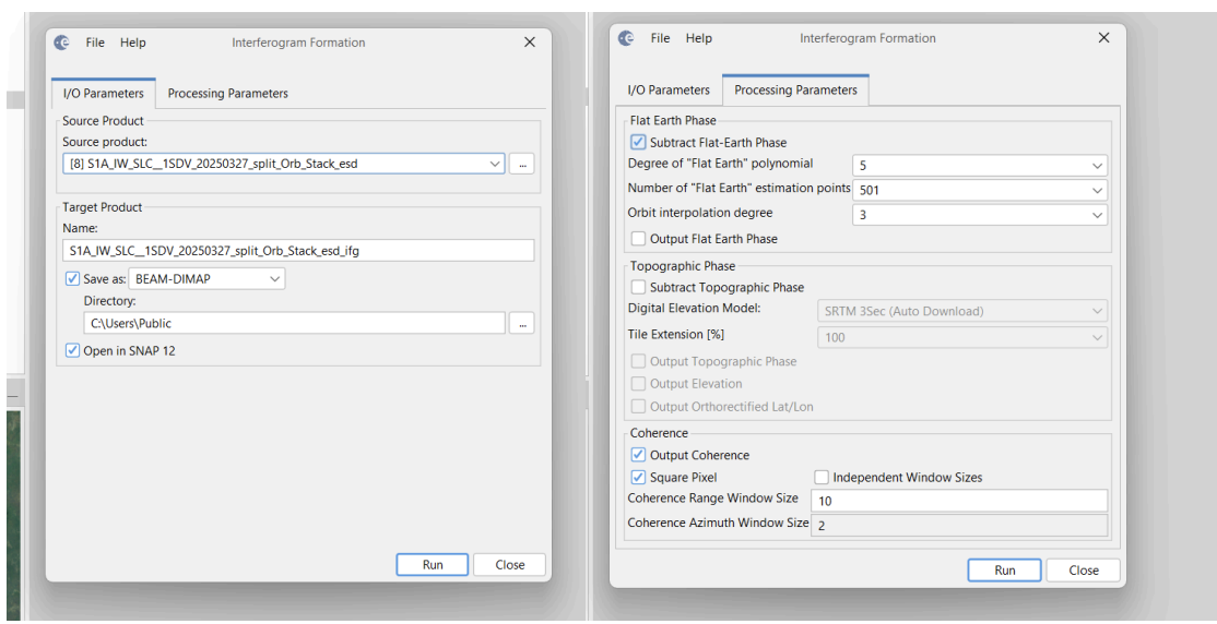
Fig 3.7 Selecting the Co-registered stack as input for the Interferogram Formation

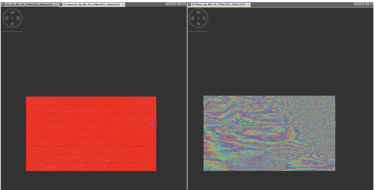
Fig 3.8 Screenshot of the generated Interferogram Phase difference and Intensity

Step 6 — TOPSAR Deburst

In order to remove the burst boundaries in the phase difference by seamlessly joining all bursts in the swath into a single image, I applied the TOPSAR Deburst process next on the interferogram result.

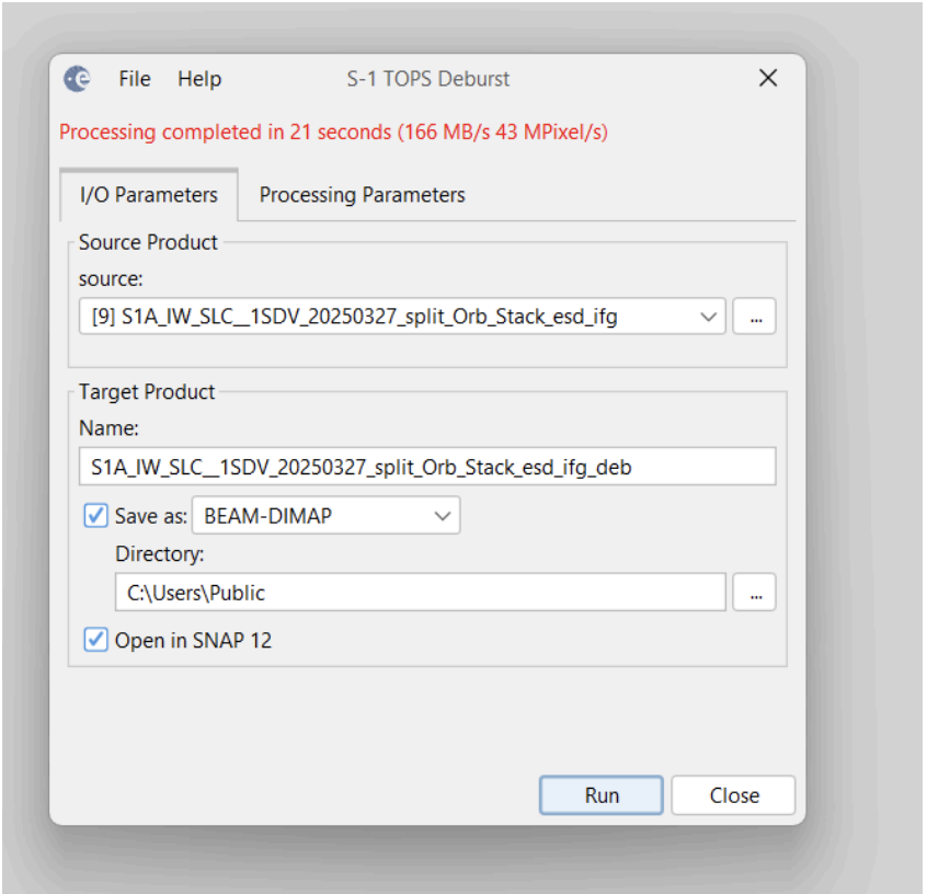
Fig 3.9 Successful Deburst process on the interferogram

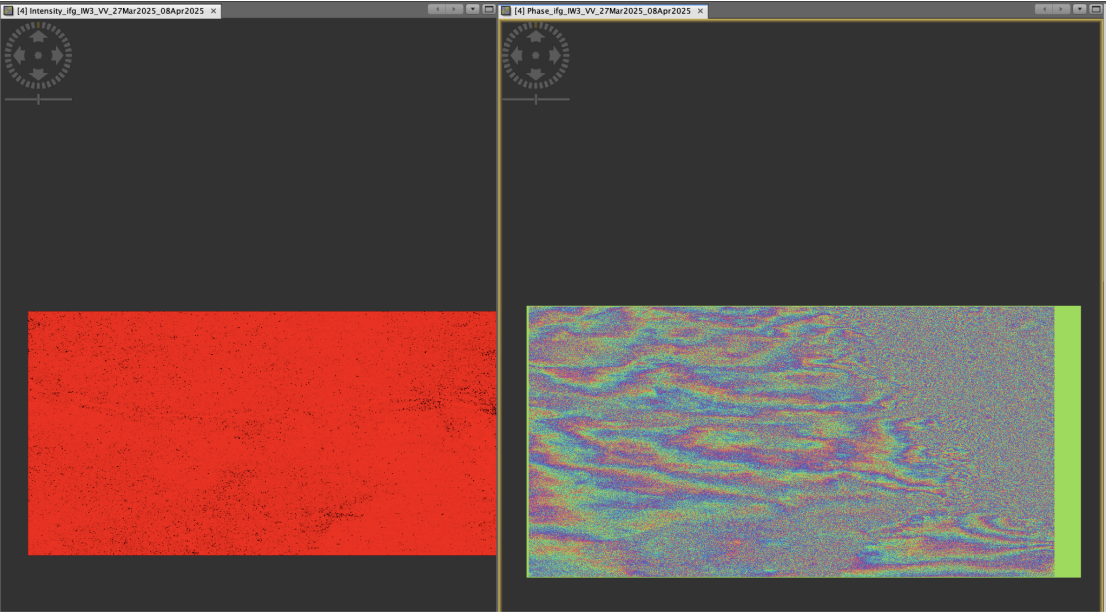
Fig 4.0 Results of the Phase difference and Intensity after the Deburst process

Step 7 — Topographic Phase Removal

To proceed to generating a differential interferogram, there is a need to remove the topographic effects. I then applied the Topographic Phase removal first to the generated topographic interferogram. For the phase removal configuration, I changed the Digital Elevation model to "SRTM 1Sec HGT (Auto Download)" and also checked the "Output the Elevation Band" to ensure the result also has the Elevation band.

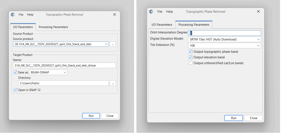
Fig 4.1 Applying Topographic Phase Removal to the Interferogram

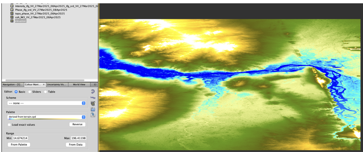
Fig 4.2 Elevation Band

Step 8 — Multilooking

This next step reduces noise and most importantly used to get square pixels and this would improve the visual interpretability of the differential interferogram. To configure the process, to get square pixels. I changed the of range looks to 8 and this change automatically calculated the Mean GR Square Pixel to 27.3680584.

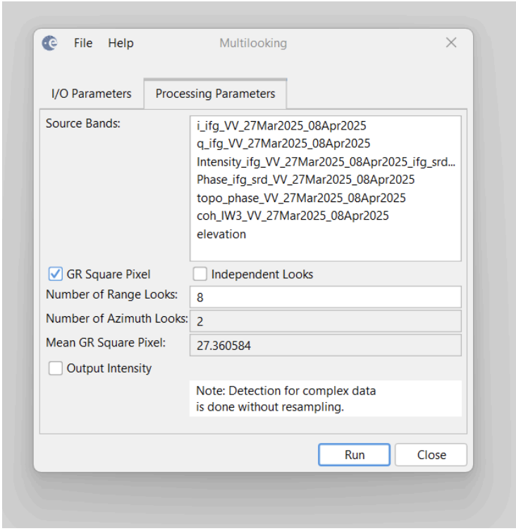
Fig 4.3 Configuring Multilooking parameter

Step 9 — Goldstein Phase Filtering

The Goldstein phase filtering is an important process to ensure phase quality by reducing noise and preparing the phase for accurate unwrapping and displacement calculation at the end. To perform the Goldstein phase filtering, I used a coherence threshold of 0.9 to reduce the noise perfectly as it seems to do a perfect noise reduction in the result.

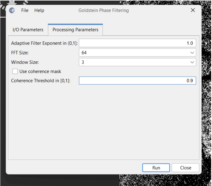
Fig 4.4 Applying the Goldstein phase filtering of coherence threshold of 0.9

Step 10 — SNAPHU Export

This stage is crucial to perform phase unwrapping with the SNAPHU plugin though the command line. I created an export folder and used the SNAPHU Export tool in the Phase Unwrapping option to export the phase.

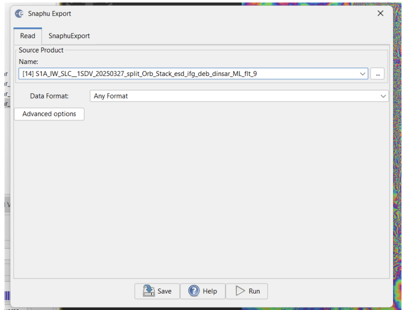
Fig 4.5 Selected the Goldstein Phase filtered result for SNAPHU export

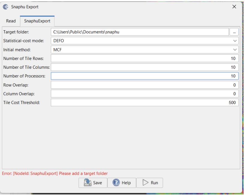
Fig 4.6 Selected the Target folder for the SNAPHU export

Step 11 — Edited the SNAPHU Configuration File

In the exported folder, I located the snaphu .conf file and edited the file with the following:

• Commented out the LOGFILE line
• Pasted the coherence file name in the OUTFILE line
• Saved the .conf file after edit

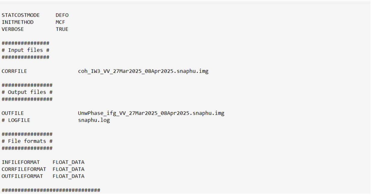
Fig 4.7 Editing the snaphu .conf file to perform the phase unwrapping

Step 12 — Run SNAPHU for Phase Unwrapping

Opened the terminal in the export folder directory and entered the following command to perform the phase unwrapping.

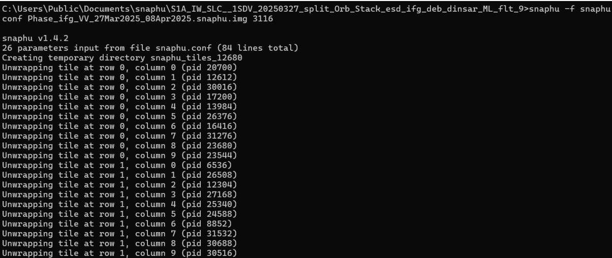
Fig 4.8 SNAPHU phase unwrapping command execution

The Phase unwrapping took just 61 seconds to complete because of the computer processor.

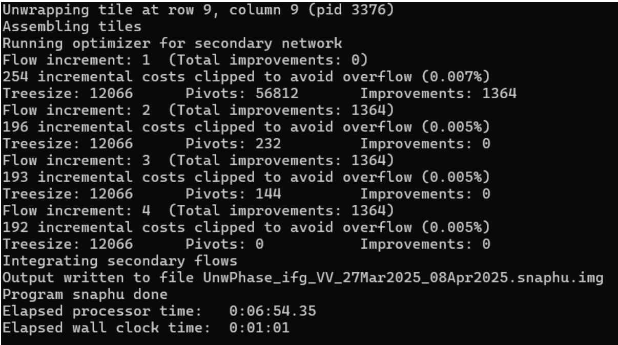
Fig 4.9 SNAPHU phase unwrapping completion

Step 13 — SNAPHU Import of the Unwrapped Phase

The unwrapped phase result in the was imported into the SNAP platform by the SNAPHU import tool which required that I selected the original product i.e the interferogram after the application of the Goldstein Phase Filtering in the 1-Read phase tab and the unwrapped phase file in the 2-Read Unwrapped Phase tab.

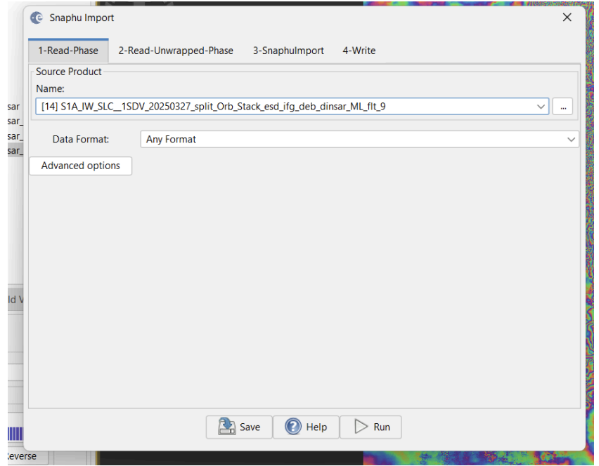
Fig 5.0 Selected the Original interferogram phase (Wrapped Phase)

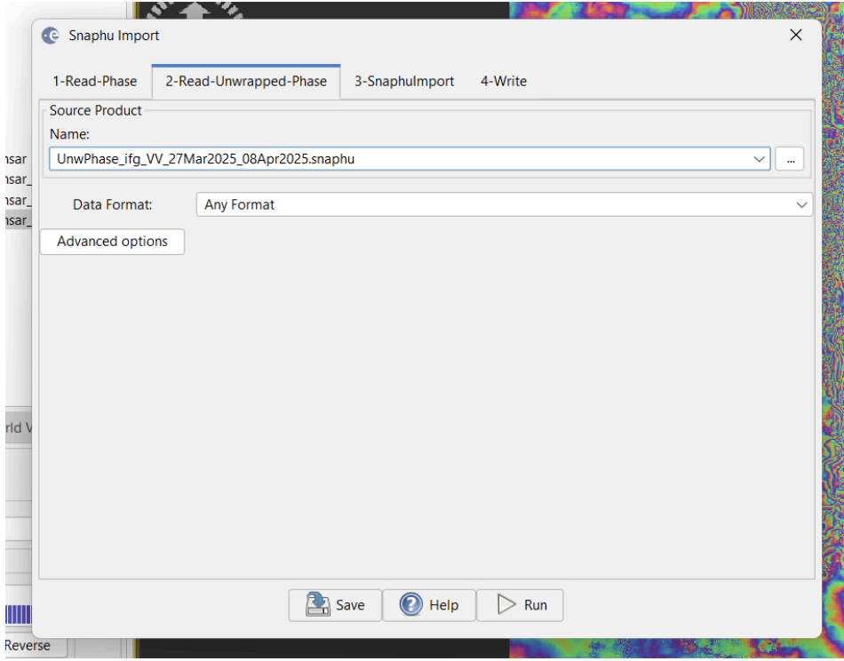
Fig 5.1 Importing the Unwrapped phase into SNAP using SNAPHU Import

Step 14 — Generate Displacement

Once the unwrapped phase is back in SNAP, we can finally translate those signal shifts into a meaningful Displacement Map. By using the Phase to Displacement tool, it converted the unwrapped phase data into actual measurements of ground shift. This will allow proper visualization and analysis of the exact scale of the terrain deformation resulting from the earthquake.

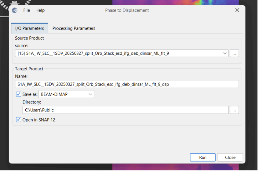
Fig 5.2 Converting the Unwrapped phase to Displacement

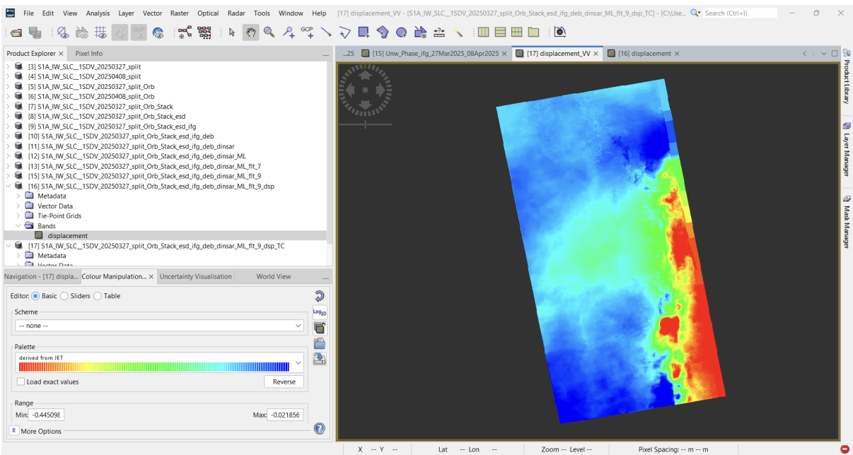
Fig 5.3 Displacement Map

Step 15 — Range-Doppler Terrain Correction

This is the final step of the interferometry analysis which georeferences the displacement map to a coordinate system and removes all distortions caused by the topography.

Fig 5.4 Configuring the Range-Doppler Terrain Correction

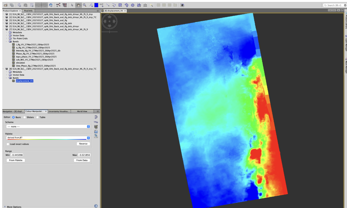
Fig 5.5 Displacement Map after the Terrain correction

Discussion & Interpretation

The InSAR analysis of the Sentinel-1 Radar Image revealed a significant deformation pattern across the fault line. The displacement map shows values ranging from -0.02 m to -0.444 m. The maximum displacement of 44.4 cm (away from the satellite) was concentrated along the western side of the fault rupture. This high magnitude of displacement was a direct result of the 7.7 magnitude earthquake, which caused the crust to rupture and settle. The negative values indicates that the side of the fault experienced a combination of downward subsidence and horizontal shifting.

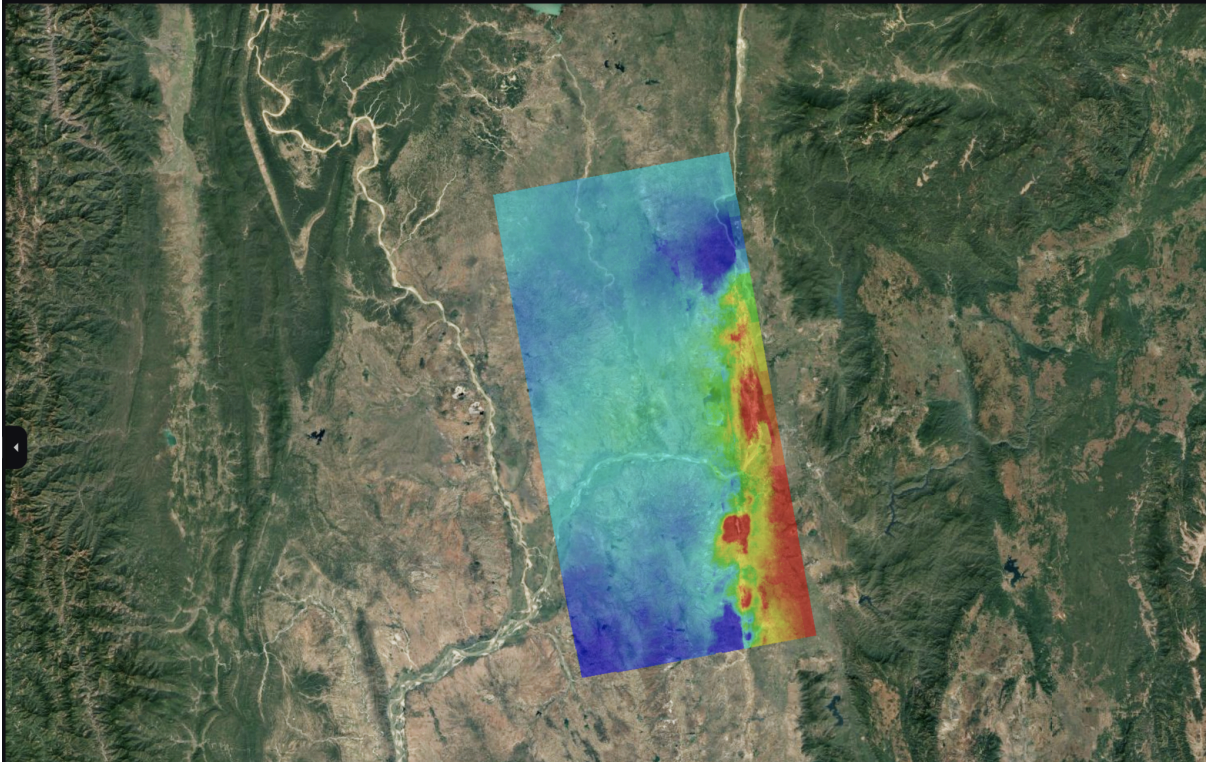
Fig 5.6 Visualization of the displacement map on Google Earth Pro

References

• BBC News (2025) 'Myanmar earthquake: Powerful 7.7 magnitude tremor strikes', BBC News, 28 March. Available at: https://www.bbc.com/news/articles/crlxlxd7882o (Accessed: 23 December 2025).
• Copernicus (2025) S1 Mission Polarimetry. Available at: https://sentiwiki.copernicus.eu/web/s1-mission#S1-Mission-Polarimetry (Accessed: 23 December 2025).
• Hussain, S., Pan, B., Hussain, W., Ali, M., Sajjad, M. M., Afzal, Z. and Tariq, A. (2025) 'Analyzing coseismic displacement of the M 7.7 Myanmar earthquake on March 28, 2025, using Sentinel-1 InSAR data', Structures, 80, 109718. doi: 10.1016/j.istruc.2025.109718.
• Wikipedia (2025) 2025 Myanmar earthquake. Available at: https://en.wikipedia.org/wiki/2025_Myanmar_earthquake (Accessed: 23 December 2025).